
Exploring Daft's Local Execution: The Swordfish Engine
Explore how Daft's Rust-powered engine executes DataFrame and SQL queries. Learn how Swordfish enables fast, streaming image processing at scale.
by ByteDance Volcano Engine, Colin HoDaft is a high-performance data engine providing simple and reliable data processing for any modality and scale, supporting both single-node and distributed execution modes. Its core is written in Rust and provides both Python DataFrame and SQL interfaces.
In the article Processing 300K Images Without OOM: A Streaming Solution, we demonstrated how Daft can easily handle streaming processing of large-scale image datasets. But how does Daft execute a user-submitted DataFrame or SQL behind the scenes? In this post, we'll continue using image processing as our entry point, diving deep into Daft's single-node execution engine through a typical image classification DataFrame example.
Use case: Image Classification
Using the images from the ImageNet dataset, we want to classify the images into categories. With Daft, we can define our processing logic in the following steps.
- Read the Parquet dataset and filter for images with 256-pixel height and width.
- Download image binary data from URLs and decode them.
- Preprocess images including cropping and normalization.
- Run inference with ResNet50 model, returning similarity labels.
- Write results as a new image dataset in Lance format.
Here's the core implementation:
df = (daft
      # Read Parquet image dataset
      .read_parquet(
"s3://daft-public-datasets/imagenet/sample_100k/data")
      # Filter for target dimensions
      .filter((col('height') == 256) & (col('width') == 256))
      # Download image bytes via URL
      .with_column('bytes', col('url').url.download())
      # Decode bytes into image type
      .with_column('image', col('bytes').image.decode(mode=ImageMode.RGB)).exclude('bytes')
      # Apply basic preprocessing (crop, normalize, etc.)
      .with_column('tensor', col('image').apply(
        func=lambda img: transform(img),
        return_dtype=daft.DataType.tensor(dtype=daft.DataType.float32()))).exclude("image")
      # Run inference with ResNet50 for offline labeling
      .with_column('labels', ResNetModel(col('tensor'))).exclude('tensor')
      .limit(100)
      )

df.write_lance(
    uri="/tmp/output"
)
Daft's Layered Architecture
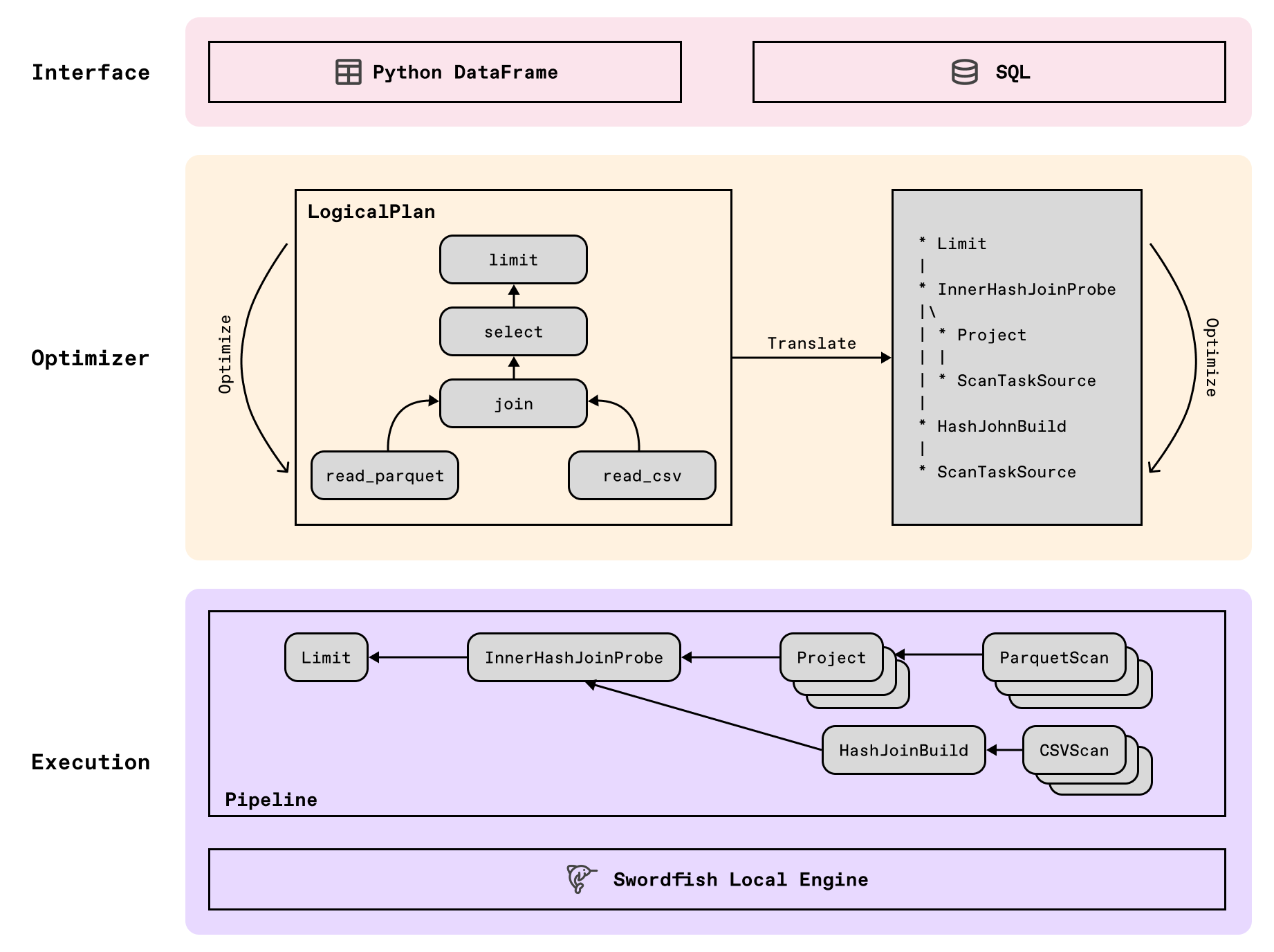
Before analyzing the DataFrame execution, let's understand Daft's layered architecture. Beyond the local or distributed runtime environment, Daft's architecture consists of three layers:
-
API Layer: Daft provides both a Python DataFrame API and SQL interface that abstracts distributed multimodal data into tabular form. Simply store images / videos / documents as columns in a table, and operate on them as you would any other column.
-
Plan Layer: Daft internally converts user DataFrame/SQL input into logical plans for unified representation, applies optimizers for better performance, then transforms the optimized logical plan into a physical plan.
-
Execution Layer: The optimized physical plan is translated into a pipeline, which is then executed in a streaming fashion by the Swordfish engine.
In addition to single node execution, Daft also provides distributed execution, allowing seamless scaling without rewriting code. See documentation to learn more about running distributed.
From DataFrame to Optimized Logical Plan
User-defined DataFrame applications are internally represented as logical execution plan trees. Daft's LogicalPlanBuilder constructs these from DataFrames. For our example, the unoptimized logical plan looks like:
* Limit: 100
|
* Project: col(name), col(height), col(width), col(url), col(labels)
|
* Project: col(name), col(height), col(width), col(url), col(tensor), py_udf(col(tensor)) as labels
|
[... multiple Project nodes ...]
|
* Filter: [col(height) == lit(256)] & [col(width) == lit(256)]
|
* GlobScanOperator
|   Glob paths = [s3://ai/dataset/url_ILSVRC2012/*.parquet]
|   File schema = name#Utf8, height#Int64, width#Int64, url#Utf8
While our DataFrame doesn't use select for column filtering, multiple Project nodes appear because with_column operations add columns via built-in operators or UDFs. Internally, Daft uses Project nodes to represent with_column semantics.
Since LogicalPlanBuilder's construction is essentially a "literal translation" process, directly executing this plan would be inefficient. Like traditional compute engines, Daft implements an optimizer framework with dozens of rules to rewrite logical plans.
Key optimizations applied to our example include:
-
Filter/Limit Pushdown: Pushes filter (256x256) and limit (100) expressions to the Scan node, reducing data scanned and processed.
-
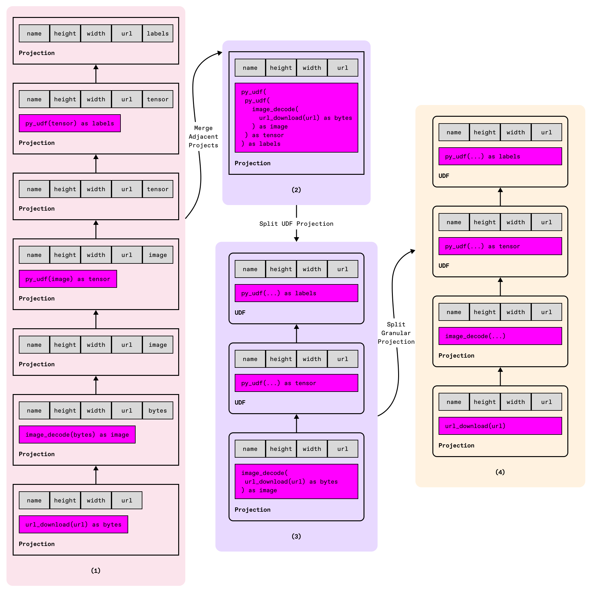
Projection Folding: Combines consecutive Project nodes into one, shortening execution paths and enabling expression pushdown.
-
UDF Separation: Splits UDF projections from regular projections for more control over batch sizing and concurrency. This also allows Daft to run them on separate Python processes for parallelism without being GIL bound.
-
Fine-grained Project Splitting: Particularly for url_download expressions - instead of processing 10,000 URLs in one task (risking OOM and connection limits), this enables finer control over batch size and concurrency.
The optimized logical plan becomes:
* UDFProject:
|   UDF __main__.ResNetModel = py_udf(col(__TruncateRootUDF_0-4-0__)) as labels
|   Concurrency = Some(4)
|   Resource request = { num_cpus = 0, num_gpus = 0.25 }
|
[... intermediate nodes ...]
|
* Num Scan Tasks = 1424
|   Filter pushdown = [col(height) == lit(256)] & [col(width) == lit(256)]
|   Limit pushdown = 100
|   Stats = { Approx num rows = 300,469, Approx size bytes = 16.23 MiB }
Beyond these rules, Daft's optimizer includes many others like CrossJoin/Subquery/Repartition elimination, predicate pushdown, column pruning, and Join reordering, continuously evolving.
From Logical Plan to Physical Plan
The optimized logical plan still represents the DataFrame's logical semantics and can't be directly executed. Logical plans focus on "what to do" while physical plans address "how to do it" - including execution platform and single vs. distributed mode.
The physical plan for our example:
* UDF Executor:
|   UDF __main__.ResNetModel = py_udf(col(0: __TruncateRootUDF_0-4-0__)) as labels
|   Concurrency = 4
|   Resource request = { num_cpus = 0, num_gpus = 0.25 }
|
[... intermediate operators ...]
|
* ScanTaskSource:
|   Num Scan Tasks = 1424
|   Pushdowns: {filter: [col(height) == lit(256)] & [col(width) == lit(256)], limit: 100}
|   Schema: {name#Utf8, height#Int64, width#Int64, url#Utf8}
For single-node execution, converting logical to physical plans essentially involves depth-first traversal and one-to-one operator mapping. Not all logical operators have physical counterparts - for instance, Offset is rewritten as Limit at the optimizer level.
Executing with Swordfish
Swordfish uses a pipeline streaming architecture implemented in Rust, leveraging the Tokio async runtime for async non blocking I/O and a multithreaded work scheduler.
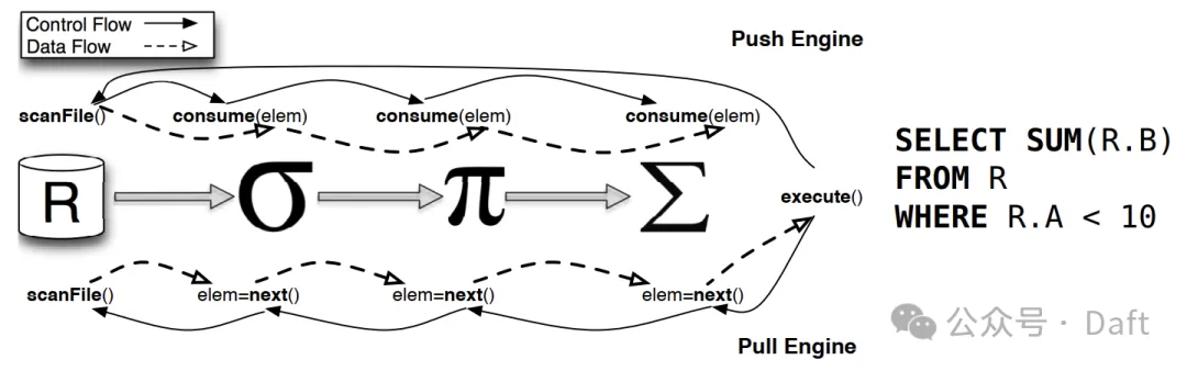
Unlike the classic Volcano model's iterator-based Pull approach, Swordfish adopts a Morsel-driven Push model. Once pipeline nodes start, source nodes begin running Scan tasks to load data, which is split into small morsels and passed between nodes via async channels for streaming processing.
Building the Pipeline
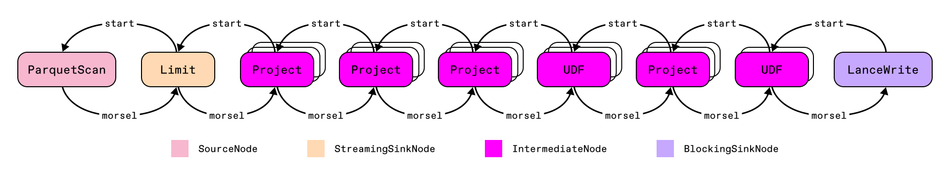
Swordfish converts physical plans into pipelines using four node types:
| Node Type | Role | Concurrency | Operator Examples |
|---|---|---|---|
| SourceNode | Data source | Dependent on CPU cores and scan task statistics | PhysicalScan |
| IntermediateNode | Processing | Operator-specific, default CPU cores | Project, Filter, UDF |
| BlockingSinkNode | Blocking sink | Operator-specific, default CPU cores | Aggregate, Repartition, WriteSink |
| StreamingSinkNode | Streaming sink | Operator-specific, default CPU cores | Limit, Concat, MonotonicallyIncreasingId |
The pipeline for our example:
Executing the Pipeline
To initiate execution, Swordfish traverses the pipeline tree depth-first, calling each node's start method. The leaf nodes then begin producing data, pushing them up to subsequent operators via async channels.
Swordfish uses the Tokio async runtime to manage concurrent scheduling of compute and IO. Tokio provides a seamless API to perform async non-blocking I/O, which is especially important when downloading from cloud storage. Furthermore, its multithreaded work scheduler also serves as a good framework for concurrent compute execution. Operators schedule work across threads via Tokio tasks, and Tokio can interleave tasks across operators via the work scheduler.
To manage memory, backpressure is maintained via dynamic batch sizing, as well as bounded async channels. This allows for stable memory usage even with datasets larger than memory.
Referenced from "Processing 300K Images Without OOM," used only to illustrate data flow in the Pipeline, not representing the data processing flow of the example DataFrame
Let's explore three key questions about pipeline execution:
1. How is data loaded?
During plan construction and optimization, Daft creates ScanTasks, usually one per file. These ScanTasks stream data at the morsel granularity to the downstream nodes. To prevent resource contention from thousands of concurrent ScanTasks, Daft maintains a task pool limiting concurrent executions.
2. How is data processed?
Taking UDF execution as an example, our DataFrame defines two UDFs:
transform: Stateless UDF for row-wise image preprocessing.ResNetModel: Stateful UDF that loads ResNet50 at initialization and processes images in batches.
IntermediateNode encapsulates UDFs in the pipeline. Upon startup, it:
- Calculates worker concurrency based on UDF's concurrency parameter (defaulting to CPU cores).
- Chunks or splits upstream morsels based on
batch_sizeparameter. - Submits morsels to UDF workers on separate threads or processes, which execute the UDF logic.
3. How is data written back?
Daft has several data connectors to write data out. In the image classification example, we write to local disk in the Lance format. Swordfish streams PyArrow Tables directly into the Lance writer. Since both use Arrow's memory model, data moves zero-copy from compute to storage. Writes are pipelined with computation, so batches are flushed as they're produced, overlapping I/O with compute work and keeping resources fully utilized.
Conclusion
In this post, we:
- Introduced Daft's three-layer architecture from a macro perspective.
- Used an image classification DataFrame example to analyze how Daft builds and optimizes logical plans, then transforms them into physical plans.
- Explored how Swordfish constructs pipelines from physical plans and executes them in a streaming fashion.
While one article can't cover every detail of Daft's internals, this overview provides a foundation for deeper exploration of Daft's implementation.
Check us out on Github, follow us on LinkedIn, join us on Slack, and pip install daft to get started.
References
- Morsel-driven parallelism: a NUMA-aware query evaluation framework for the many-core age
- Push versus pull-based loop fusion in query engines
- Efficiently compiling efficient query plans for modern hardware
Read the original blog posts in Chinese:

