
Scaling As-of Joins
How we built, broke, and re-built our ASOF joins — 6x faster, half the memory of pandas, and scaled to a distributed cluster.
by Euan LimDaft now offers native ASOF joins, an operation essential for aligning time series data, such as sensor streams that tick at different rates. In this post, I'll walk through how we implemented ASOF joins, made them 6x faster, and cut memory usage in half. We'll dive into the three optimizations behind the wins (hash grouping, binary search, and multi-threaded parallelism) and show how the same architecture scales out to a distributed cluster.
But first, what is an ASOF join?
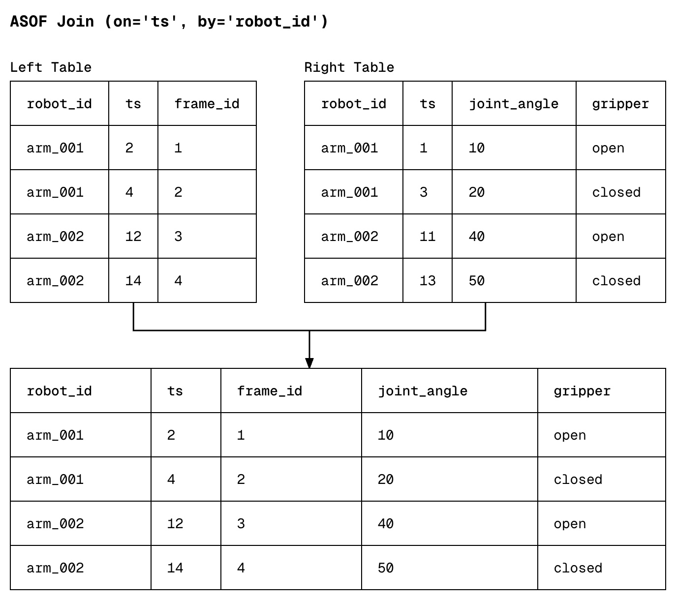
ASOF joins link two datasets by matching each timestamp in one table with the most recent timestamp in another table. In the example below, data collected in the left and right table do not align perfectly, and an ASOF join simply tries to answer the question "for each video frame, what was the latest joint angle & gripper state of our robot?"
How to perform an ASOF join
To perform an ASOF join in Daft, use the .join_asof() method.
on: the column to match on (usually a timestamp).by: the column to partition by, so rows only match within the same entity (e.g. samerobot_id).
import daft

frames = daft.from_pydict(
    {
        "ts": [2, 5, 8],
        "robot_id": ["arm_001", "arm_001", "arm_002"],
        "frame_id": [1, 2, 3],
    }
)

telemetry = daft.from_pydict(
    {
        "ts": [1, 4, 8],
        "robot_id": ["arm_001", "arm_001", "arm_002"],
        "joint_angle": [10.0, 20.0, 30.0],
        "gripper": ["open", "closed", "open"],
    }
)

result = frames.join_asof(telemetry, on="ts", by="robot_id", strategy="backward")
result.show()| ts | robot_id | frame_id | joint_angle | gripper |
|---|---|---|---|---|
| 2 | arm_001 | 1 | 10 | open |
| 5 | arm_001 | 2 | 20 | closed |
| 8 | arm_002 | 3 | 30 | open |
Building V1: Sort + two-pointers
Our first implementation of an ASOF join was a sorted two-pointer search.
- Sort the left and right tables by a composite
(by, on)key. This groups rows by entity and orders them by timestamp within each entity. - Walk both tables with two pointers. For each left row, advance the right pointer through rows of the same
bykey as long asright.ts <= left.ts. The last such right row is the match.
Benchmarking V1
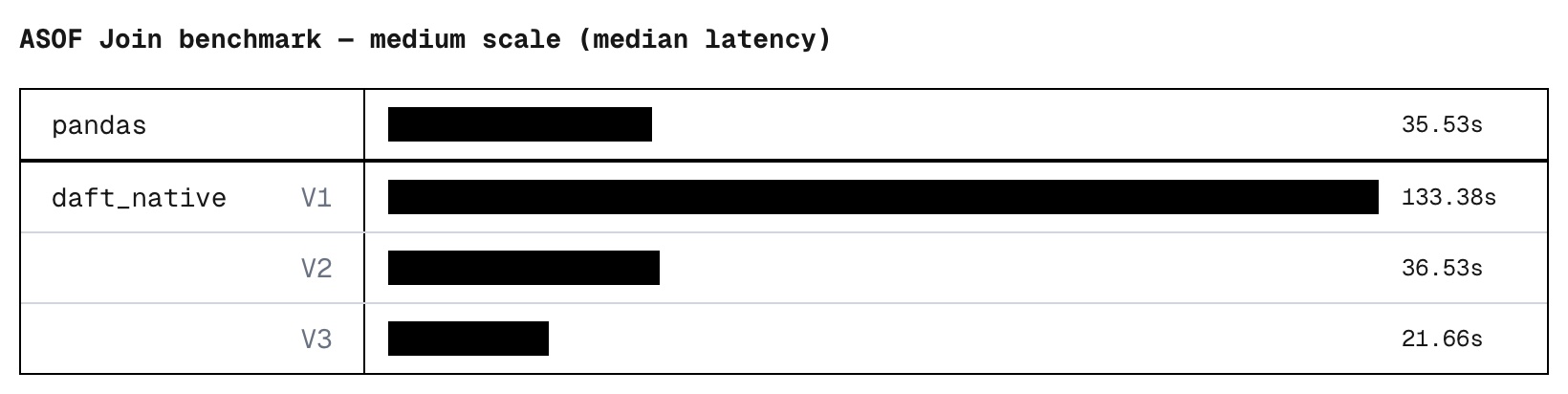
We benchmarked this initial implementation against pandas on a synthetic workload (10M left rows, 100M right rows) and discovered that were 3.75x slower.
system       scale    status   med_time_s  med_peak_gb
pandas       medium   ok            35.53         9.08

V1
daft_native  medium   ok           133.38        10.28
Profiling the run revealed to us that we were bottlenecked by our string comparisons. While integer comparison takes a single CPU cycle, comparing strings involved an iteration through memory character by character. Furthermore, ASOF joins allow users to specify multiple "by" keys, each requiring a computationally expensive string-matching operation.

This broke our assumption that a simple sort and two-pointer approach would easily work, even though it was O(M log M + N log N) (where M and N represent the number of rows in your left and right table respectively). Big O tells you how your algorithm scales, but not how much each operation costs.

Building V2: Parallel hash bucketing + two pointers
Given that the bottleneck was caused by a multi-key string comparison during sorting, we wanted our new implementation to elide this completely. Here's what we came up with:
- Hash the left & right tables by their "by" keys to group rows belonging to the same entity together
- Parallelize the sorting of each entity's left and right table by their "on" keys
- Do the same two-pointer approach within each entity
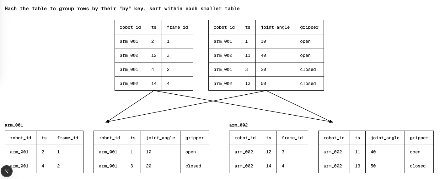
Previously, every comparison made while sorting included expensive string columns, potentially multiple of them. By switching to hash grouping, we had a much cheaper way to partition our data. Within each group, we'd now only need to sort by the "on" key, which was a single (typically integer) column. Not only is each comparison cheaper, since we had already grouped the tables by their "by" key, we could parallelize the sorting of each group across cores, giving us a significant performance increase.
system       scale    status   med_time_s  med_peak_gb
pandas       medium   ok            35.53         9.08

V1
daft_native  medium   ok           133.38        10.28

V2
daft_native  medium   ok            36.53        10.58
Building V3: Streaming ASOF Joins
Still, V2's parallelism model had a fundamental flaw. It was based on the number of "by" key groups, which meant that parallelism was dependent on your data cardinality. If you had a 32-core machine but only 2 "by" keys, you'd only ever use 2 cores while the other 30 sit idle.
Furthermore, our previous approach required us to materialize both the left and right table before doing any computation. We weren't leveraging the streaming nature of the Daft engine, which would have allowed us to process batches of the right table incrementally. We decided to take a different approach for V3:
The Build Phase
- Materialize all rows from the left table
- Group rows of the same "by" key together and sort each group by their "on" key
- Build a hash map over the groups, enabling O(1) lookups
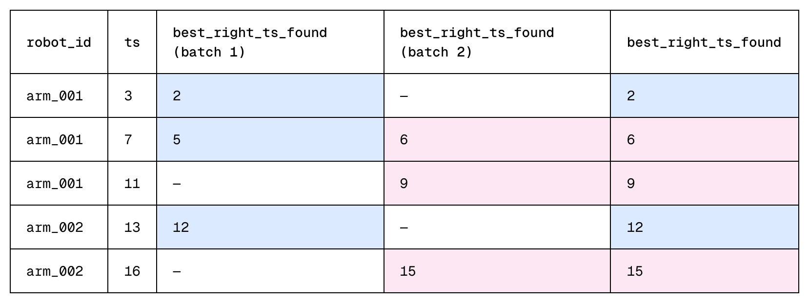
The Probe Phase
- The right table streamed into the Daft engine in equal sized batches. Each batch is treated as its own, independent task, with each task running in parallel on a separate thread.
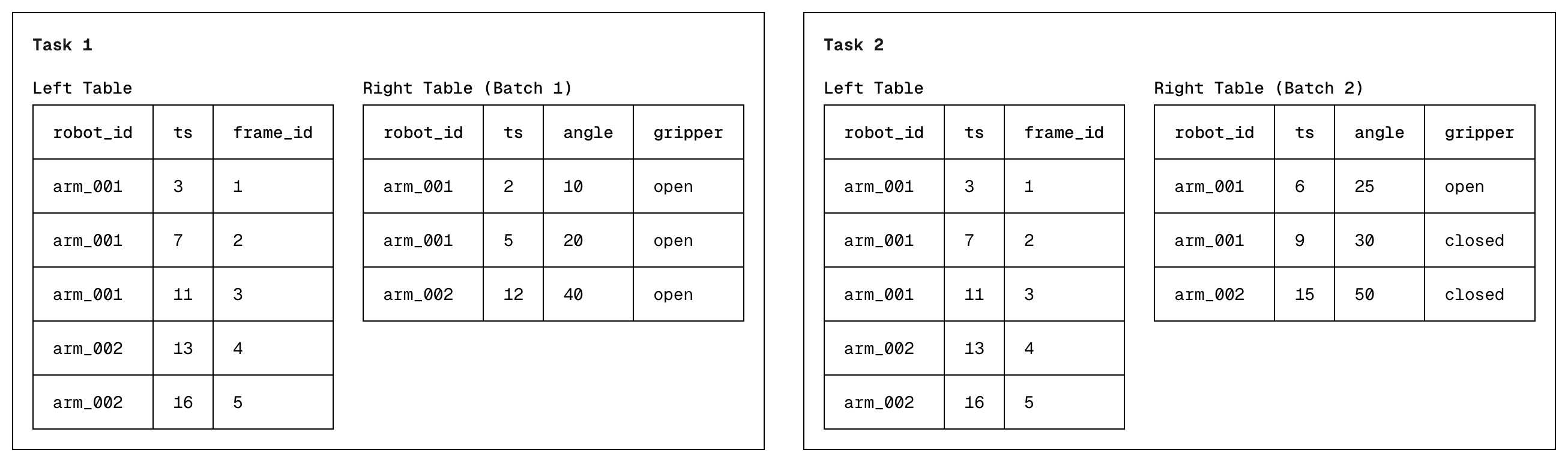
- The goal for each task is to determine, for every left table row, the best matching right table row seen within that batch via binary search. This is the first left row where the left "on" key >= right "on" key. We also use the same hash-grouping approach from V1 & V2. Each task stores its own results, allowing them to run in parallel.
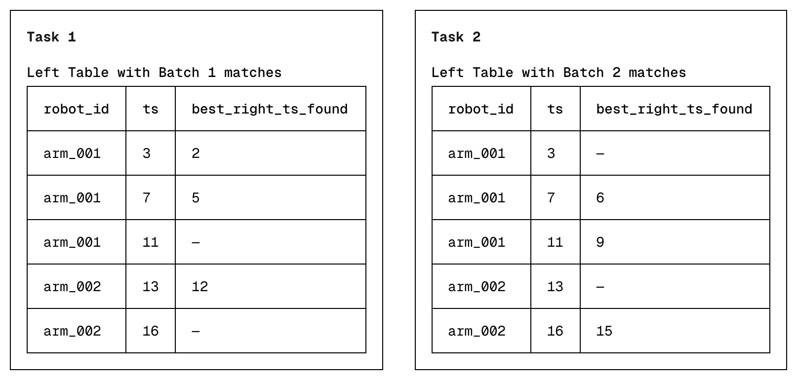
- Once all tasks complete, each left row may have multiple compatible rows from each independent task. During the final merge step, we pick the best compatible right row across all tasks.
Why is V3 Better?
In V2, parallelism was determined by your data cardinality. You got one parallel unit per "by" key group, and nothing more.
In V3, parallelism doesn't depend on your data cardinality at all. Regardless of your number of "by" keys, it is able to process batches of the right table in parallel. Two "by" keys on a 32-core machine are no longer restricted to just 2 cores. The resolution step follows the same principle. Rather than a single sequential merge, left rows are chunked across cores and resolved in parallel. Finally, with a streaming approach, we are also able to push more work earlier into the pipeline, rather than waiting for all the data to materialize.
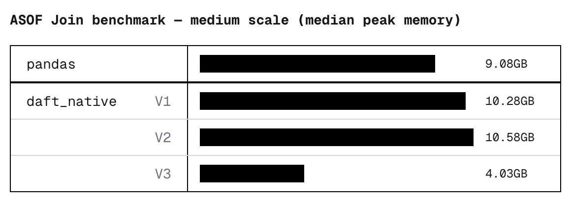
For the cherry on top, we also threw in a couple of memory optimizations: Unnecessary columns are pruned from the right tables as early as possible, and candidate results are tracked using lightweight pointers instead of copies of the data.
The result: A native ASOF join that optimizes for speed while minimizing its memory footprint.
Going Distributed
Some datasets simply cannot fit into the RAM of even the most powerful machine. One day's worth of robotics data can include 1-10TB of video data and 5-500GB of sensor data. Running an ASOF join of this scale on your laptop simply isn't possible. Scaling ASOF joins to the next level required making it work performantly on a distributed Daft cluster.
Why hash-partitioning wouldn't work
We initially considered the same hash-then-sort pattern in V2. Rows of the same entity & "by" key would go to the same worker, and each worker could process each entity in parallel. This approach introduced two critical bottlenecks.
First, if a user does not specify a grouping "by" key, the hashing logic defaults to a single worker, forcing all rows back onto a single worker.
Secondly, real-world data rarely follows a uniform distribution — one robot might generate ten times more data than another — leading to the problem of Data Skew. When certain keys appear orders of magnitude more frequently than others, whichever node draws these hot keys becomes a bottleneck while the rest of the cluster sits idle. And because wall-to-wall timing is always dictated by your slowest node, this "long tail" latency negates the benefits of scaling.
V4: Range Partitioned ASOF joins
To combat data skew, we move away from hash-based partitioning towards a range based partitioning system. Here's how it works:
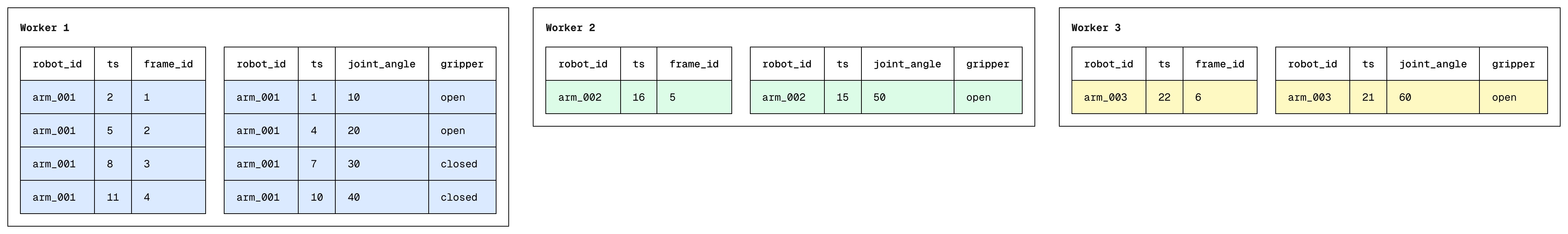
Sampling & Range Partitioning
We'd first sample composite (by, on) keys from the left & right table to estimate the global key distribution. Using the sample, we compute N-1 range boundaries (for N workers) and shuffle both tables so each worker gets one partition. All rows in partition i are strictly less than those in partition i+1, with roughly equal data volume per partition.
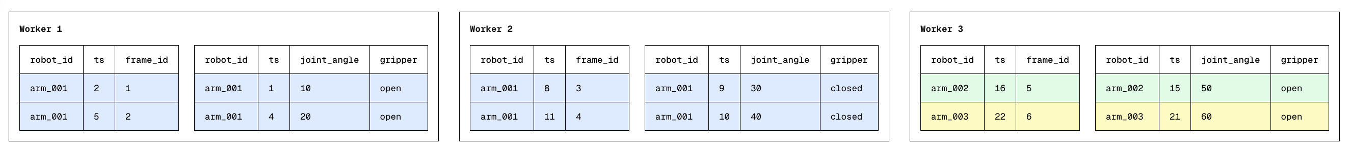
Dispatching "Carryovers"
Distributing data volume evenly across workers requires us to consider some edge cases: What if we had multiple "by" keys on the same node, or a single "by" key distributed across nodes? How would we perform an ASOF join then?
Turns out, the only modification to our original algorithm would be to ensure that each worker has a "memory" of what happened immediately before its own data starts. We call this a Carryover. In a globally sorted dataset, an ASOF join only looks "backwards." This means that even if a single "by" key is split across multiple different nodes, the only requirement for correctness is for worker i+1 to know the single most recent record in the right table of worker i.
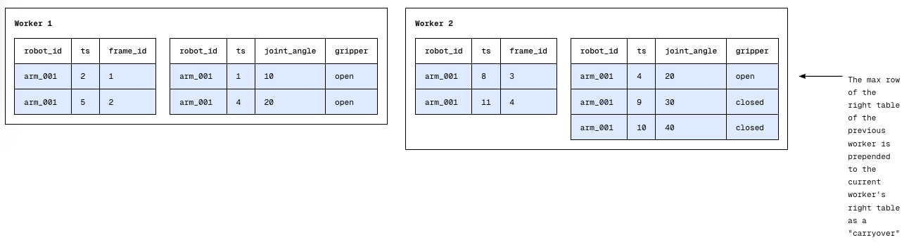
Local ASOF Join
As long as each worker pre-pends the carryover to its right table, this allows the standard two-pointer merge to run locally. We are guaranteed that even if the "closest match" for a row existed on a different physical machine, the carryover has brought that data where it needs to be.
The result is a distributed ASOF join that scales horizontally even if data was skewed — no hotspots, no long-tail latency, no single worker dragging down the entire query.
Try it out yourself
Distributed ASOF joins sit at the intersection of several hard problems — efficiency, memory pressure, skew resistance, and correctness across partition boundaries. If you're building physical AI pipelines or ML feature stores, you shouldn't have to solve them yourself.
We already did. Give it a try!
import daft

frames = daft.from_pydict(
    {
        "ts": [2, 5, 8],
        "robot_id": ["arm_001", "arm_001", "arm_002"],
        "frame_id": [1, 2, 3],
    }
)

telemetry = daft.from_pydict(
    {
        "ts": [1, 4, 8],
        "robot_id": ["arm_001", "arm_001", "arm_002"],
        "joint_angle": [10.0, 20.0, 30.0],
        "gripper": ["open", "closed", "open"],
    }
)

result = frames.join_asof(telemetry, on="ts", by="robot_id", strategy="backward")
result.show()| ts | robot_id | frame_id | joint_angle | gripper |
|---|---|---|---|---|
| 2 | arm_001 | 1 | 10 | open |
| 5 | arm_001 | 2 | 20 | closed |
| 8 | arm_002 | 3 | 30 | open |
We welcome your feedback on these features! Let us know how we can improve Daft and what you would like to see, by submitting an issue on Github or sending us a message on our community Slack.
Appendix
Data Generation
Schema
Each table — left and right — shares an identical three-column schema:
| Column | Type |
|---|---|
ts | int64 |
entity | utf8 |
val | float64 |
Size
Datasets are generated at three scale tiers. The right table is always 10× larger than the left, reflecting the pattern where a lookup/reference table dwarfs the probe table in an ASOF join (e.g. video frames as the ts-indexed left table, joined against denser sensor telemetry on the right)
| Scale | Left rows | Right rows | Left files | Right files |
|---|---|---|---|---|
| Small | 1 M | 10 M | 1 | 2 |
| Medium | 10 M | 100 M | 2 | 20 |
| Large | 50 M | 500 M | 10 | 100 |
Each Parquet file targets ~256 MB (5 M rows). Files are Snappy-compressed.
Entity Distribution
There are 10,000 distinct entities (e00000–e09999). Entity assignments follow a Zipf distribution with exponent (s = 1.0), meaning the most frequent entity appears roughly 10,000× more often than the least frequent one. This intentional skew stresses join implementations that do not account for hot-key imbalance.
Benchmarks
All single node benchmarks were ran on a r7i.2xlarge EC2 instance
system       scale    status   med_time_s  med_peak_gb
pandas       medium   ok            35.53         9.08

V1
daft_native  medium   ok           133.38        10.28

V2
daft_native  medium   ok            36.53        10.58

V3
daft_native  medium   ok            21.66         4.03
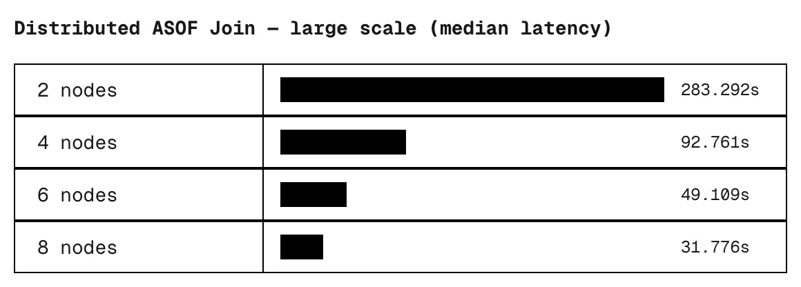
All distributed benchmarks were run on r7i.4xlarge EC2 instances
scale  nodes  status  med_time_s
large  2      ok      283.29
large  4      ok       92.76
large  6      ok       49.11
large  8      ok       31.78

